In this post, we looked at the network discovery process overall. Here, we'll dive into how exactly automated network assurance can change this process. Traditionally, you'd rely on a time-consuming manual process that will result in a High-Level Design (HLD) document, Low-Level Design document (LLD), access credentials, a list of devices with access information, and more. However, the IP Fabric approach can flip how you view this necessary information. Are static documents really an effective way of documenting a large and complex enterprise network? Why not rely on dynamically updated documentation that comprehensively captures your network state at a point in time, using no hours or effort from your engineers?
To contrast two methods of discovering the network - manual vs IP Fabric - let's use a simple High-Level Design doc as our case study. We'll assume:
Now that we have all the information we need, let’s start discovering the network.
Please note that this whole lab is virtual and based on the IOL devices; therefore the switch is identified as “linux_l2” and router as “linux-l3.”
So that we can see how beneficial IP Fabric is, we’ll need to go over the traditional manual method of discovering a network.
The manual method is an old concept that shouldn’t be used on the kind of networks we’re dealing with — large and complex networks. However, it may very well be the method you're stuck with today. To start, use a device list that looks like this:
After that, we need to log into the first known device so that we can connect with other devices, starting with the ones closest to the center. Use commands to:
Every node needs to be checked, and every adjacent device should be noted for later examination. The short video below shows the beginning of this manual process.
It’s blatantly evident that this approach is very time-consuming and isn’t feasible for large, complex networks. When creating a proper network diagram, all active interfaces need to be documented, and each device needs to be drawn in relation to neighboring devices throughout the whole network.
Your mileage may vary, but analyzing all the active nodes and filling out the table above took us approximately 45 minutes, drawing the network diagram took somewhere around an additional 30 minutes.
Today, businesses see the value in automating repetitive tasks to save time, which in turn cuts costs. There are plenty of methods that can be used to simplify the network discovery — you could, for example, use your own scripts and very simple tools like NMAP or BASH scripting, then use some management protocol, like SNMP (shown below).
The example above shows two phases — getting the IP addresses, then gathering the specific data from these SNMP-activated hosts through a simple script.
Compiling a list of active devices with a specific IP can be done a few different ways — you can ping the entire subnet (as the HLD stated all the IP addresses are from the 172.16/12 subnet), or you can use a Nmap command can make it more effective.
root@tom-linuxmint:~/lab# nmap -sn -n --host-timeout 2s 172.31.100.0/24 | grep Nmap
Starting Nmap 7.60 ( https://nmap.org ) at 2018-12-31 08:58 CET
Nmap scan report for 172.31.100.1
Nmap scan report for 172.31.100.2
Nmap scan report for 172.31.100.3
Nmap scan report for 172.31.100.4
Nmap scan report for 172.31.100.5
Nmap scan report for 172.31.100.6
Nmap scan report for 172.31.100.7
Nmap scan report for 172.31.100.8
Nmap scan report for 172.31.100.9
Nmap scan report for 172.31.100.10
Nmap scan report for 172.31.100.11
Nmap scan report for 172.31.100.51
Nmap scan report for 172.31.100.52
Nmap scan report for 172.31.100.53
Nmap scan report for 172.31.100.54
Nmap scan report for 172.31.100.55
Nmap scan report for 172.31.100.60
Nmap scan report for 172.31.100.61
Nmap scan report for 172.31.100.62
Nmap scan report for 172.31.100.63
Nmap scan report for 172.31.100.101
Nmap scan report for 172.31.100.102
Nmap scan report for 172.31.100.103
Nmap scan report for 172.31.100.104
Nmap done: 256 IP addresses (24 hosts up) scanned in 2.02 seconds
This method uses ICMP echo without any protocol probe (TCP/UDP), so a much better and more effective way would be to check some specific protocol availability. For example, TCP/22 and TCP/23 can be used to test the Telnet and SSH port and UDP/161 to check SNMP port, as shown below:
root@tom-linuxmint:~/lab# nmap -sU -p 161 172.31.100.0/24 | grep Nmap
Starting Nmap 7.60 ( https://nmap.org ) at 2018-12-31 10:20 CET
Nmap scan report for 172.31.100.1
Nmap scan report for 172.31.100.2
Nmap scan report for 172.31.100.3
Nmap scan report for 172.31.100.4
Nmap scan report for 172.31.100.5
Nmap scan report for 172.31.100.6
Nmap scan report for 172.31.100.7
Nmap scan report for 172.31.100.8
Nmap scan report for 172.31.100.9
Nmap scan report for 172.31.100.10
Nmap scan report for 172.31.100.11
Nmap scan report for 172.31.100.51
Nmap scan report for 172.31.100.52
Nmap scan report for 172.31.100.53
Nmap scan report for 172.31.100.54
Nmap scan report for 172.31.100.55
Nmap scan report for 172.31.100.60
Nmap scan report for 172.31.100.61
Nmap scan report for 172.31.100.62
Nmap scan report for 172.31.100.63
Nmap scan report for 172.31.100.101
Nmap scan report for 172.31.100.102
Nmap scan report for 172.31.100.103
Nmap scan report for 172.31.100.104
Nmap done: 256 IP addresses (24 hosts up) scanned in 3.96 seconds
Nmap is checking to see if the UDP/161 is open or not since there isn’t any SNMP specific check with the community or version test. These outputs are returning the same set of IP addresses, but in the real network, these lists can be different since not all active devices can be managed through the SNMP.
This BASH script uses the previous list of devices as an input data and processes each item as follows:
#!/bin/bash
filename='lab-active-devices'
echo Start
while read p; do
  if snmpget -v2c -c labnet $p iso.3.6.1.2.1.1.1.0 | grep -q 'Cisco'; then
    vendor="Cisco"
    hostname=`snmpget -v2c -c labnet $p iso.3.6.1.2.1.1.5.0 | awk '{print $4}'`
    ios=`snmpget -v2c -c labnet $p iso.3.6.1.2.1.1.1.0 | grep Software | awk '{print $9}'`
  fi
  echo "$p, ${hostname:1:-1}, $vendor", ${ios:1:-2}
done < $filename
The only function executed is checking SNMP OID for sysDescr to test if it’s a Cisco device or not. It can be extended for other vendors if needed, but it’s enough for this lab to distinguish between a Cisco and non-Cisco device. The function then uses sysName for the device hostname and again uses the sysDescr to get the IOS version. This approach is used only for this demonstration as an illustration on how to use SNMP framework and simple scripts — the key is to know what to get and how to represent it using known tools like scripting or post-process editing tools, (like office tools, for example).
The same mechanism can be used to create a network diagram, but the Nmap should check the whole IP space, and the scripts should access all of the devices, analyzing the directly connected subnets. Pairing the devices within the same subnets creates the baseline for the network diagram and should be extended with specific IPs and interface names.
Using this process, this list of devices was created in just five minutes (instead of the 45 minutes it took compiling it the manual way). Creating scripts to gather all of the data for the network diagram took around five more minutes, and the topology was built in approximately 25 minutes.
Network discovery can be completed by a few tools that already exist, but so that you can understand the unique benefits of IP Fabric's platform, let’s take a look at the tool’s incredibly easy setup and deployment process. To get started, all you need to do is enter the credentials IP Fabric will need to access the network devices, and supply a few other details for use during the discovery process.
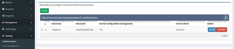
If you’d like, you can set additional parameters. We’re going to use these in our example:
Once that’s done, hit the play, sit back, and watch IP Fabric get to work (example shown below).
The entire process is automatic, without any interaction from you needed, and IP Fabric saves all data that it generates for further analysis and graphical presentation.
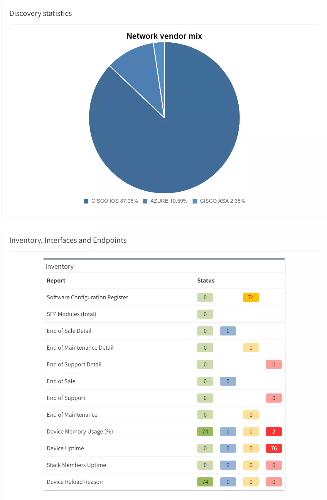
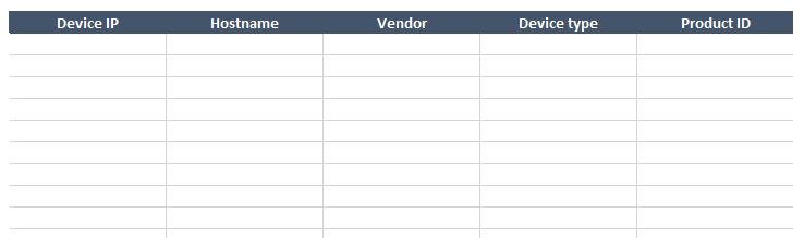
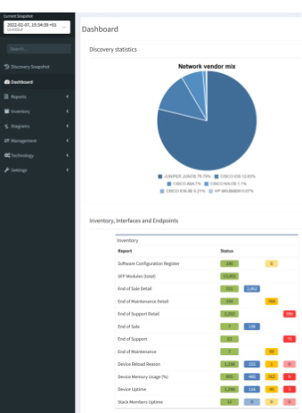
The first part of the results that you should check is the inventory list (shown below). Compare the list IP Fabric generated to the one you created manually, to see if any differences exist. It shocks many users when they see results on the IP Fabric list that escaped their eye when they built the list manually.
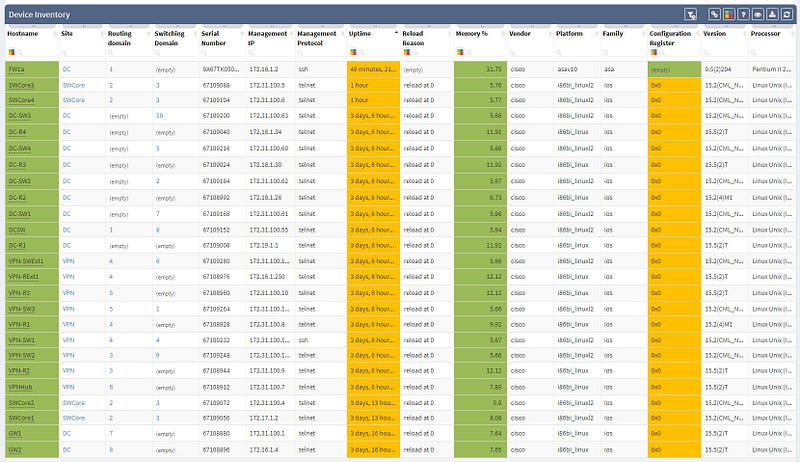
As you can see, the list shows a significant amount of network device details, including vendor information, management IP address, software version, and even additional information like uptime, memory usage, etc. Not only does this help us validate our assumptions, but it provides additional helpful information, which helps expand our knowledge base.
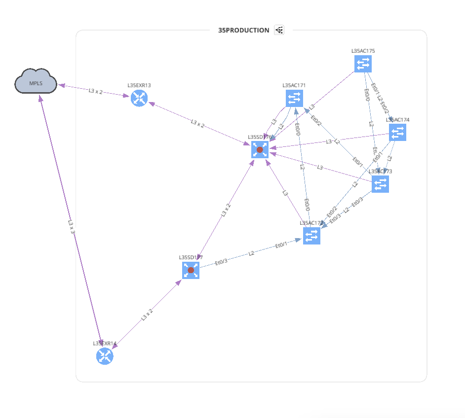
The next part of IP Fabric’s results that you should check is the network diagram graphic.
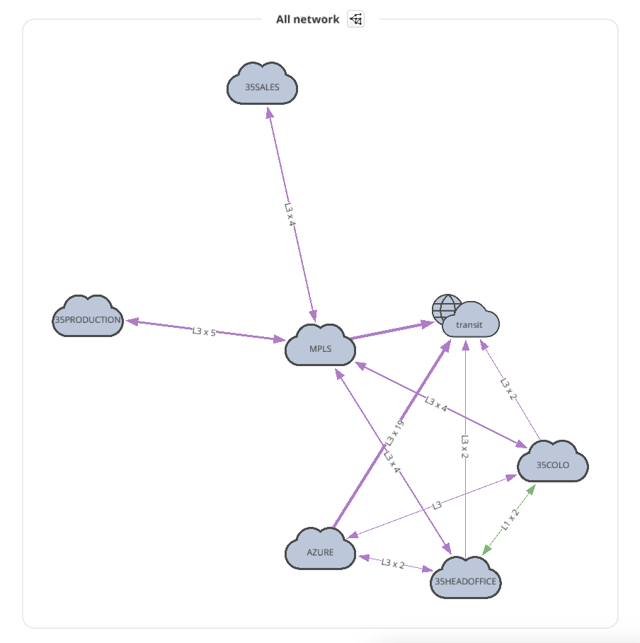
The diagram visually groups the devices based on site name (you can adjust the site naming convention in the discovery settings with regexp string). It’s not a diagram of the practical look of the network, but IP Fabric offers ways of modifying the diagram by clicking the cloud images, hiding site boundaries, showing (or hiding) the L2/L3 connections, etc. With these features, you can use IP Fabric to create a diagram closer to the real topology, like the one shown below.
Now that we’ve covered how quick and easy it is to deploy and use IP Fabric, making it the obvious choice when discovering unknown networks, you’re ready to try it out for yourself.
Lastly, we’re going to delve into more great ways that IP Fabric can help simplify your work life, so keep an eye out for more parts of this series.
To learn more about how IP Fabric’s platform can help you with analytics or intended network behavior reporting, feel free to get in touch with the team, or try our self-guided demo!
In this post, we looked at the network discovery process overall. Here, we'll dive into how exactly automated network assurance can change this process. Traditionally, you'd rely on a time-consuming manual process that will result in a High-Level Design (HLD) document, Low-Level Design document (LLD), access credentials, a list of devices with access information, and more. However, the IP Fabric approach can flip how you view this necessary information. Are static documents really an effective way of documenting a large and complex enterprise network? Why not rely on dynamically updated documentation that comprehensively captures your network state at a point in time, using no hours or effort from your engineers?
To contrast two methods of discovering the network - manual vs IP Fabric - let's use a simple High-Level Design doc as our case study. We'll assume:
Now that we have all the information we need, let’s start discovering the network.
Please note that this whole lab is virtual and based on the IOL devices; therefore the switch is identified as “linux_l2” and router as “linux-l3.”
So that we can see how beneficial IP Fabric is, we’ll need to go over the traditional manual method of discovering a network.
The manual method is an old concept that shouldn’t be used on the kind of networks we’re dealing with — large and complex networks. However, it may very well be the method you're stuck with today. To start, use a device list that looks like this:
After that, we need to log into the first known device so that we can connect with other devices, starting with the ones closest to the center. Use commands to:
Every node needs to be checked, and every adjacent device should be noted for later examination. The short video below shows the beginning of this manual process.
It’s blatantly evident that this approach is very time-consuming and isn’t feasible for large, complex networks. When creating a proper network diagram, all active interfaces need to be documented, and each device needs to be drawn in relation to neighboring devices throughout the whole network.
Your mileage may vary, but analyzing all the active nodes and filling out the table above took us approximately 45 minutes, drawing the network diagram took somewhere around an additional 30 minutes.
Today, businesses see the value in automating repetitive tasks to save time, which in turn cuts costs. There are plenty of methods that can be used to simplify the network discovery — you could, for example, use your own scripts and very simple tools like NMAP or BASH scripting, then use some management protocol, like SNMP (shown below).
The example above shows two phases — getting the IP addresses, then gathering the specific data from these SNMP-activated hosts through a simple script.
Compiling a list of active devices with a specific IP can be done a few different ways — you can ping the entire subnet (as the HLD stated all the IP addresses are from the 172.16/12 subnet), or you can use a Nmap command can make it more effective.
root@tom-linuxmint:~/lab# nmap -sn -n --host-timeout 2s 172.31.100.0/24 | grep Nmap
Starting Nmap 7.60 ( https://nmap.org ) at 2018-12-31 08:58 CET
Nmap scan report for 172.31.100.1
Nmap scan report for 172.31.100.2
Nmap scan report for 172.31.100.3
Nmap scan report for 172.31.100.4
Nmap scan report for 172.31.100.5
Nmap scan report for 172.31.100.6
Nmap scan report for 172.31.100.7
Nmap scan report for 172.31.100.8
Nmap scan report for 172.31.100.9
Nmap scan report for 172.31.100.10
Nmap scan report for 172.31.100.11
Nmap scan report for 172.31.100.51
Nmap scan report for 172.31.100.52
Nmap scan report for 172.31.100.53
Nmap scan report for 172.31.100.54
Nmap scan report for 172.31.100.55
Nmap scan report for 172.31.100.60
Nmap scan report for 172.31.100.61
Nmap scan report for 172.31.100.62
Nmap scan report for 172.31.100.63
Nmap scan report for 172.31.100.101
Nmap scan report for 172.31.100.102
Nmap scan report for 172.31.100.103
Nmap scan report for 172.31.100.104
Nmap done: 256 IP addresses (24 hosts up) scanned in 2.02 seconds
This method uses ICMP echo without any protocol probe (TCP/UDP), so a much better and more effective way would be to check some specific protocol availability. For example, TCP/22 and TCP/23 can be used to test the Telnet and SSH port and UDP/161 to check SNMP port, as shown below:
root@tom-linuxmint:~/lab# nmap -sU -p 161 172.31.100.0/24 | grep Nmap
Starting Nmap 7.60 ( https://nmap.org ) at 2018-12-31 10:20 CET
Nmap scan report for 172.31.100.1
Nmap scan report for 172.31.100.2
Nmap scan report for 172.31.100.3
Nmap scan report for 172.31.100.4
Nmap scan report for 172.31.100.5
Nmap scan report for 172.31.100.6
Nmap scan report for 172.31.100.7
Nmap scan report for 172.31.100.8
Nmap scan report for 172.31.100.9
Nmap scan report for 172.31.100.10
Nmap scan report for 172.31.100.11
Nmap scan report for 172.31.100.51
Nmap scan report for 172.31.100.52
Nmap scan report for 172.31.100.53
Nmap scan report for 172.31.100.54
Nmap scan report for 172.31.100.55
Nmap scan report for 172.31.100.60
Nmap scan report for 172.31.100.61
Nmap scan report for 172.31.100.62
Nmap scan report for 172.31.100.63
Nmap scan report for 172.31.100.101
Nmap scan report for 172.31.100.102
Nmap scan report for 172.31.100.103
Nmap scan report for 172.31.100.104
Nmap done: 256 IP addresses (24 hosts up) scanned in 3.96 seconds
Nmap is checking to see if the UDP/161 is open or not since there isn’t any SNMP specific check with the community or version test. These outputs are returning the same set of IP addresses, but in the real network, these lists can be different since not all active devices can be managed through the SNMP.
This BASH script uses the previous list of devices as an input data and processes each item as follows:
#!/bin/bash
filename='lab-active-devices'
echo Start
while read p; do
  if snmpget -v2c -c labnet $p iso.3.6.1.2.1.1.1.0 | grep -q 'Cisco'; then
    vendor="Cisco"
    hostname=`snmpget -v2c -c labnet $p iso.3.6.1.2.1.1.5.0 | awk '{print $4}'`
    ios=`snmpget -v2c -c labnet $p iso.3.6.1.2.1.1.1.0 | grep Software | awk '{print $9}'`
  fi
  echo "$p, ${hostname:1:-1}, $vendor", ${ios:1:-2}
done < $filename
The only function executed is checking SNMP OID for sysDescr to test if it’s a Cisco device or not. It can be extended for other vendors if needed, but it’s enough for this lab to distinguish between a Cisco and non-Cisco device. The function then uses sysName for the device hostname and again uses the sysDescr to get the IOS version. This approach is used only for this demonstration as an illustration on how to use SNMP framework and simple scripts — the key is to know what to get and how to represent it using known tools like scripting or post-process editing tools, (like office tools, for example).
The same mechanism can be used to create a network diagram, but the Nmap should check the whole IP space, and the scripts should access all of the devices, analyzing the directly connected subnets. Pairing the devices within the same subnets creates the baseline for the network diagram and should be extended with specific IPs and interface names.
Using this process, this list of devices was created in just five minutes (instead of the 45 minutes it took compiling it the manual way). Creating scripts to gather all of the data for the network diagram took around five more minutes, and the topology was built in approximately 25 minutes.
Network discovery can be completed by a few tools that already exist, but so that you can understand the unique benefits of IP Fabric's platform, let’s take a look at the tool’s incredibly easy setup and deployment process. To get started, all you need to do is enter the credentials IP Fabric will need to access the network devices, and supply a few other details for use during the discovery process.
If you’d like, you can set additional parameters. We’re going to use these in our example:
Once that’s done, hit the play, sit back, and watch IP Fabric get to work (example shown below).
The entire process is automatic, without any interaction from you needed, and IP Fabric saves all data that it generates for further analysis and graphical presentation.
The first part of the results that you should check is the inventory list (shown below). Compare the list IP Fabric generated to the one you created manually, to see if any differences exist. It shocks many users when they see results on the IP Fabric list that escaped their eye when they built the list manually.
As you can see, the list shows a significant amount of network device details, including vendor information, management IP address, software version, and even additional information like uptime, memory usage, etc. Not only does this help us validate our assumptions, but it provides additional helpful information, which helps expand our knowledge base.
The next part of IP Fabric’s results that you should check is the network diagram graphic.
The diagram visually groups the devices based on site name (you can adjust the site naming convention in the discovery settings with regexp string). It’s not a diagram of the practical look of the network, but IP Fabric offers ways of modifying the diagram by clicking the cloud images, hiding site boundaries, showing (or hiding) the L2/L3 connections, etc. With these features, you can use IP Fabric to create a diagram closer to the real topology, like the one shown below.
Now that we’ve covered how quick and easy it is to deploy and use IP Fabric, making it the obvious choice when discovering unknown networks, you’re ready to try it out for yourself.
Lastly, we’re going to delve into more great ways that IP Fabric can help simplify your work life, so keep an eye out for more parts of this series.
To learn more about how IP Fabric’s platform can help you with analytics or intended network behavior reporting, feel free to get in touch with the team, or try our self-guided demo!